Kurtosis refers to the measurement of the degree to which a given distribution is more or less ‘peaked’ relative to the normal distribution. The concept of kurtosis is very useful in decision-making. In this regard, we have 3 categories of distributions:

• Leptokurtic;
• Mesokurtic; or
• Platykurtic.

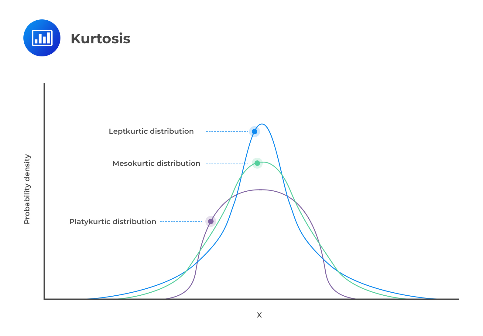
Leptokurtic

A leptokurtic distribution is more peaked than the normal distribution. The higher peak results from the clustering of data points along the x-axis. The tails are also fatter than those of a normal distribution. The coefficient of kurtosis is usually more than 3.

The term “lepto” means thin or skinny. When analyzing historical returns, a leptokurtic distribution means that small changes are less frequent since historical values are clustered around the mean. However, there are also large fluctuations represented by the fat tails.

Platykurtic

A platykurtic distribution has extremely dispersed points along the x-axis, resulting in a lower peak when compared to a normal distribution. “Platy” means broad. Hence, the prefix fits the distribution’s shape, which is wide and flat. The points are less clustered around the mean compared to a leptokurtic distribution. The coefficient of kurtosis is usually less than 3.

Returns that follow this type of distribution have fewer major fluctuations compared to leptokurtic returns. However, you should note that fluctuations represent the riskiness of an asset. More fluctuations represent more risk and vice versa. Therefore, platykurtic returns are less risky than leptokurtic returns.

Mesokurtic

Lastly, mesokurtic distributions have a curve that is similar to that of a normal distribution. In other words, the distribution is largely normal.

Measures of Sample Skewness and Kurtosis

Exam tip: The learning outcome statement reads, “explain measures of sample skewness and kurtosis.” However, the calculations will have you better understand those concepts.

Sample Skewness

Sk=1n∑ni=1(Xi−¯X)3S3

Where:

¯X = Sample mean;

S = Sample standard deviation; and

n = Number of observations.

Note: The formula is very similar to the formula for standard deviation, but raised to the 3rd power.

Interpretation: A positive value indicates positive skewness. A ‘zero’ value indicates that the data is not skewed. Lastly, a negative value indicates negative skewness or rather a negatively skewed distribution.

Sample Kurtosis

Sample kurtosis is always measured relative to the kurtosis of a normal distribution, which is 3. Therefore, we are always interested in the “excess“ kurtosis, i.e.,

 Excess kurtosis = Sample kurtosis – 3 , where:

Skr=1n∑ni=1(Xi−¯X)4S4

Interpretation: Positive excess kurtosis indicates a leptokurtic distribution. A zero value indicates a mesokurtic distribution. Lastly, a negative excess kurtosis represents a platykurtic distribution.

Example: Calculating Skewness

Suppose we have the following observations:

{ 12   13   54   56   25 }

What is the skewness of the data?

Solution

First, we must determine the sample mean and the sample standard deviation:

X=(12+13+…+25)5=1605=32

S2=(12–32)2+…+(25–32)24=467.5

Therefore,

S=467.512=21.62

Now we can work out the skewness:

Sk=1n∑ni=1(Xi−¯X)3S3=15−203+(−193)+223+243+(−73)21.623=0.1835

Skewness is positive. Hence, the data has a positively skewed distribution.

Example: Calculating Kurtosis

Using the data from the example above { 12   13   54   56   25 }, determine the type of kurtosis present.

Solution

X=(12+13+…+25)5=1605=32

S2=(12–32)2+…+(25–32)24=467.5

Therefore,

S=467.512=21.62

Skr=1n∑ni=1(Xi−¯X)4S4=15−204+(−194)+224+244+(−74)21.624=0.7861

Next, we subtract 3 from the sample kurtosis and get the excess kurtosis:

Excess kurtosis=0.7861–3=−2.2139

Since the excess kurtosis is negative, we have a platykurtic distribution.